Using the Dynamic Linear Model (dlm) package and the excellent book by Petris, Petrone and Campagnoli here is an example of dynamic regression using a simple DLM.
In case you’re not familiar with DLMs they assume that one models observables (such as prices, GDP etc.) and hidden state variables separately and that the dynamics of any problem are through the evolution of the state variables. The observables are a simple transform of the state variables rather like Plato’s allegory of the cave.
On top is the observation equation for the observable variables \(Y_t\) and below is the state equation for the state variables \(\theta_t\) which handles all the dynamics. The matrix \(F\) transforms the state variables \(\theta\) into observable variables \(Y\) and the matrix \(G\) handles the dynamics for updating \(\theta\).
\(\begin{align}
Y_t &= F_t \theta_t + v_t & v_t &\sim \mathcal{N}_m(0,V_t) & \text{ m-dimensional observation equation} \\
\theta_t &= G_t \theta_{t-1} + w_t & w_t &\sim \mathcal{N}_p(0,W_t) & \text{ p-dimensional state equation}
\end{align}
\)
The system starts off in state \(\theta_0\) but as this is itself uncertain it is specified using a Normal prior distribution centred at \(m_0\) with covariance \(C_0\) i.e. \(\theta_0 \sim \mathcal{N}_p(m_0,C_0)\).
We are going to calculate the dynamic CAPM beta for three stocks. First we get daily price series for three stocks (Apple, Microsoft, Exxon) and the “market” which we proxy with the S&P 500 tracker (SPY) and for the risk free return a Treasury ETF (IEF) all with the function get.hist.quote().
|
1 2 3 4 5 6 7 8 9 10 11 12 13 14 15 16 17 18 19 20 21 22 23 24 25 26 27 28 |
library(zoo) library(tseries) library(dlm) ticker.list <- c("SPY","AAPL","MSFT","XOM","IEF") largecapstocks <- get.hist.quote(instrument=ticker.list[1] ,start="2003-01-01" ,end=Sys.Date() ,quote="AdjClose" ,provider="yahoo" ,origin="1970-01-01" ,compression="d" ,retclass="zoo") for (ticker in ticker.list[2:length(ticker.list)]) { largecapstocks <- merge.zoo(largecapstocks ,get.hist.quote(instrument=ticker ,start="2003-01-01" ,end=Sys.Date() ,quote="AdjClose" ,provider="yahoo" ,origin="1970-01-01" ,compression="d" ,retclass="zoo")$AdjClose) colnames(largecapstocks)[ncol(largecapstocks)] <- ticker } colnames(largecapstocks)[1] <- ticker.list[1] largecapstocks <- largecapstocks[!is.na(apply(largecapstocks,1,sum)),] plot(largecapstocks) |
We need excess returns for both the market and each of the stocks
|
1 2 3 4 5 |
# excess returns are returns minus ten year Treasury returns rtns <- diff(log(largecapstocks)) y <- rtns[,c("AAPL","MSFT","XOM")] - rtns[, "IEF"] market <- rtns[, "SPY"] - rtns[, "IEF"] m <- NCOL(y) |
Then we set up and run the DLM.
|
1 2 3 4 5 6 7 8 9 10 11 12 13 14 15 16 17 |
CAPM <- dlmModReg(market) CAPM$FF <- CAPM$FF %x% diag(m) CAPM$GG <- CAPM$GG %x% diag(m) CAPM$JFF <- CAPM$JFF %x% diag(m) CAPM$W <- CAPM$W %x% matrix(0,m,m) signal.to.noise.ratio <- .5 # s/n = W / V CAPM$V <- cov(y) CAPM$W[-(1:m),-(1:m)] <- cov(y) * signal.to.noise.ratio CAPM$m0 <- rep(0,2*m) CAPM$C0 <- diag(1e7,nr=2*m) CAPMsmooth <- dlmSmooth(y,CAPM) smooth.zoo <- zoo(CAPMsmooth$s[2:nrow(CAPMsmooth$s),m+1:m],time(y)) colnames(smooth.zoo) <- colnames(y) plot(smooth.zoo,plot.type='s',col=c("red","green","blue"),xlab="",ylab="Beta to S&P 500") legend(legend=colnames(y),lty=1,col=c("red","green","blue"),x=as.Date("2010-01-01"),y=1.5) |
The end result for the betas looks like this
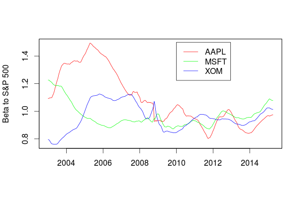
Notice the parameter “signal.to.noise.ratio”. If this is large (say around 1.0) then the data will respond more aggressively to new data and less to the estimate of the model. If the signal to noise ratio is small (around zero) the model is much less responsive to new data and the beta estimates are smoother and closer to 1.0, but they are also less responsive. There is no correct value for this parameter but it is very important in this and other examples. Try playing around with it in the example setting it to 0.01 and 1.0 and you will see the change in behaviour when you plot beta.
What this simple analysis shows is that beta for Apple and Microsoft was large in the past, well above one. Remember this is when they were small and aggressively growing and riskier enterprises. However as they have matured and grown their market cap and index weight they are much more in line with other large caps like Exxon with beta around 1. By 2008 they had effectively lost their “growth stock” status.