I’m a huge fan of the statistician Andrew Gelman. He explains statistics in such an intuitive way, and it was his book “Bayesian Data Analysis” that first opened my eyes to what is possible with Bayesian models, and how to implement them in practice. In Bayesian Data Analysis he gives many examples of hierarchical models, and since that book was written these models are much easier to implement using packages such as JAGS and Stan (see John Kruschke’s book Doing Bayesian Data Analysis for a hands-on guide).
There are many examples of data which is hierarchical. For example geographic data is often grouped hierarchically, perhaps global at the top level then grouped by country and region within a country (see Gelman’s example in Multilevel (Hierarchical) Modeling: What It Can and Cannot Do of the prevalence of radon and lung cancer rates by county in the US). A biological example would be attributes of animals or plants grouped by species, or one level up by genus, then family (see Jarrod Hadfield’s data set on Blue tits for an example). A financial example might be companies in a given country grouped by sector (for example see the paper by Pak-Wing Fok et al. on Analysis of Credit Portfolio Risk using Hierarchical Multi-Factor Models). An astrophysical example might be rates of star formation by the type of galaxy (elliptical, spiral). A business example might be employee satisfaction by business division and subdivision (see the paper by Whitener Do “high commitment” human resource practices affect employee commitment?). There are many examples from every discipline where observations are grouped in some form of hierarchy.
Here I want to explain using a simple example, which gets more complex, how to use R to build hierarchical linear models. I use a simple one dimensional data set throughout with three groups. Within each group there is a strong positive relationship between the independent variable x and the dependent variable y. However I’ve contrived the distribution such that the groups lie on a strongly negative gradient. This is how I generate the data:
- Group means are generated using a normal distribution \(\mu_{group} \sim \mathcal{N}(0,3)\)
- Group standard deviations are generated using a uniform distribution \(\sigma_{group} \sim \mathcal{U}(0.1,0.5)\)
- Intercepts for each group are generated using a negative slope which depends on the value of x \(\alpha_{group} \sim -2 \mu_{group} + \mathcal{N}(0,1)\)
- Slopes for each group are generated using a uniform distribution \(\beta_{group} \sim \mathcal{U}(0.5,1.5)\)
ngroups <- 3
groupsize <- 30

set.seed(377352)
group.x.mean <- rnorm(n = ngroups,sd=3)
group.x.sd <- runif(n = ngroups,min=0.1,max=0.5)
group.alpha <- -2 * group.x.mean + rnorm(n=ngroups,sd=1)
group.beta <- runif(n = ngroups,min = .5,max = 1.5)

group <- rep(seq(1,ngroups),each=groupsize)

# generate x and y values using group mean and sd
# for group g we use a linear function
# y = alpha[g] + beta[g] * x
# alpha[g] = -2 * x.mean[g]
# beta[g] = 1 + a tiny bit of noise
i  <- 1
x <- matrix(nrow=ngroups*groupsize)
y <- matrix(nrow=ngroups*groupsize)
for ( i.group in 1:ngroups ) {
  for ( j in 1:groupsize ) {
    x[i] <- rnorm(1,mean=group.x.mean[i.group],sd=group.x.sd[i.group])
    y[i] <- group.alpha[i.group] + group.beta[i.group] * x[i] + rnorm(1,sd=.1)
    i <- i + 1
  }
}

# if we ignore groups the gradient is negative
# this is despite the fact that each individual group
# has a gradient that is positive!
# (Intercept)        x
# -0.5472      -1.2600
library(ggplot2)
df <- data.frame(x=x,y=y,group=group)
df$group <- as.factor(df$group)
tail(df)
g <- ggplot(df) + geom_point(aes(x=x,y=y,colour=group)) +
  coord_cartesian(xlim=c(-3,1),ylim=c(-4,4)) +
  geom_smooth(aes(x=x,y=y,group=group),method=lm,se=FALSE) +
  theme_bw() + theme(legend.position="null")
g + geom_smooth(aes(x=x,y=y),method=lm,se=TRUE)
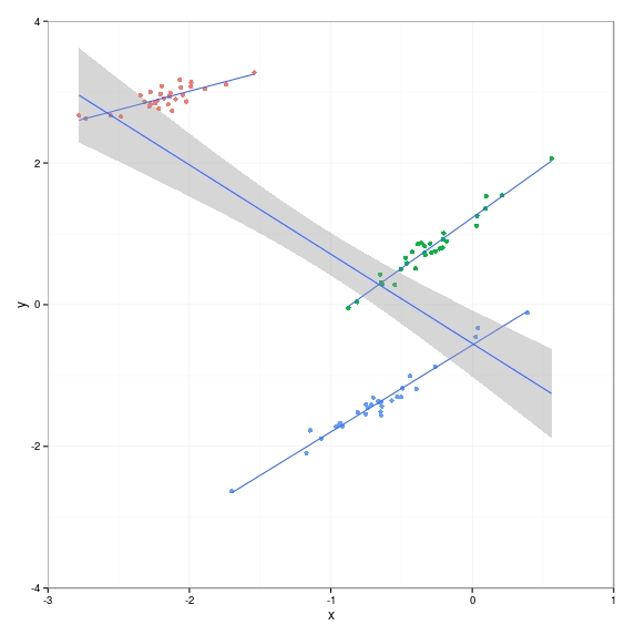
And this is what the data looks like. The groups are in different colours, you can see the positive gradients clearly. But a linear regression on all the data, ignoring the group information, erroneously fits a negative gradient. In the remainder of this post I’ll show how to model this situation with a hierarchical model that does take group information into account.
One package Gelman recommends for hierarchical linear models is arm, which has the function lmer() that works very much like the lm() function.
library(arm)
# intercept conditional on group
lmer.alpha <- lmer(y~1+x+(1|group),data=df)
# slope conditional on group
lmer.beta <- lmer(y~1+x+(x-1|group),data=df)
# both intercept and slope conditional on group
lmer.both <- lmer(y~1+x+(1+x|group),data=df) summary(lmer.alpha) summary(lmer.beta) summary(lmer.both) # fixed effect is top-level intercept and slope # (Intercept) x # 1.978652 1.144952 # group random effects on intercept # > ranef(lmer.alpha)
# $group
# (Intercept)
# 1   3.4386106
# 2  -0.8360106
# 3  -2.6026000
# > group.alpha
# [1]  4.2883814  1.2134493 -0.5410049
# > ranef(lmer.alpha)$group[,1] + fixef(lmer.alpha)[1]
# [1]  5.4172624  1.1426413 -0.6239482
fixef(lmer.alpha)
ranef(lmer.alpha)
group.alpha

# fixed effect is top-level intercept
# (Intercept)
# 5.788223
# group random effects on intercept and slope
# (Intercept)        x
# 1   -1.740225 0.518047
# 2   -4.564296 1.415710
# 3   -6.354477 1.231584
# > group.alpha
# [1]  4.2883814  1.2134493 -0.5410049
# > ranef(lmer.beta)$group + fixef(lmer.beta)[2]
# [1]  4.0479981  1.2239268 -0.5662542
fixef(lmer.beta)
ranef(lmer.beta)
group.beta

# > fixef(lmer.both)
# (Intercept)           x
# 1.578741    1.059370
# > ranef(lmer.both)
# $group
# (Intercept)          x
# 1    2.500014 -0.5272426
# 2   -0.355365  0.3545068
# 3   -2.144649  0.1727358
fixef(lmer.both)
ranef(lmer.both)

# if we have no pooling we would simply run 3 regressions, one per group
coef(lm(y~x,data=df[group==1,]))
coef(lm(y~x,data=df[group==2,]))
coef(lm(y~x,data=df[group==3,]))
# (Intercept)         x
# 4.0653645   0.5259707
# 1.227969    1.428500
# -0.570280    1.225905
# true values for group.alpha are
# 4.2883814  1.2134493 -0.5410049
(ranef(lmer.alpha)$group[,1]) + fixef(lmer.alpha)[1]
(ranef(lmer.beta)$group[,1]) + fixef(lmer.beta)[1]

# alpha model plot
fit.lines <- data.frame(cbind(intercept=(ranef(lmer.alpha)$group[,1])+fixef(lmer.alpha)[[1]]
                              ,slope=fixef(lmer.alpha)[[2]])
                        ,group=factor(1:3))
g.alpha <- g + geom_abline(aes(intercept=intercept,slope=slope,hierarchicalcolour=group),data=fit.lines) +
  ggtitle("Alpha Random Effects")
g.alpha

# beta model plot
fit.lines <- data.frame(cbind(intercept=fixef(lmer.beta)[[1]]
                              ,slope=ranef(lmer.beta)$group[,1] + fixef(lmer.beta)[1]
                              ,group=factor(1:3)))
fit.lines$group <- factor(fit.lines$group)
g.beta <- g + geom_abline(aes(intercept=intercept,slope=slope,colour=group),data=fit.lines) +
  ggtitle("Beta Random Effects")
g.beta

# both model plot
fit.lines <- data.frame(cbind(intercept=(ranef(lmer.both)$group[,1])+fixef(lmer.both)[[1]]
                              ,slope=ranef(lmer.both)$group[,2]+fixef(lmer.both)[[2]]
                              ,group=factor(1:3)))
fit.lines$group <- factor(fit.lines$group)
g.both <- g + geom_abline(aes(intercept=intercept,slope=slope,colour=group),data=fit.lines) +
  ggtitle("Alpha and Beta Random Effects")
g.both

# get this handy function from http://www.cookbook-r.com/Graphs/Multiple_graphs_on_one_page_(ggplot2)/
multiplot(g.alpha,g.beta,g.both,cols = 3)
The result is shown here. I’ve got three plots, the first where the intercept (alpha) is dependent on group, the second where slope (beta) is dependent on group and the third where both intercept and slope depend on group. You might be thinking why not just do three separate linear regressions because the third example produces coefficients very close to this. The reason is based on the assumption which is that the alphas and betas are drawn from a top-level distribution and are therefore related. This means that we can pool information between groups which becomes very important if we have very little data for one of the groups. In this case the tiny group “borrows strength” from the top-level distribution and we can still make predictions with much smaller errors than we would have for a no-pooling three-separate-regressions analysis.
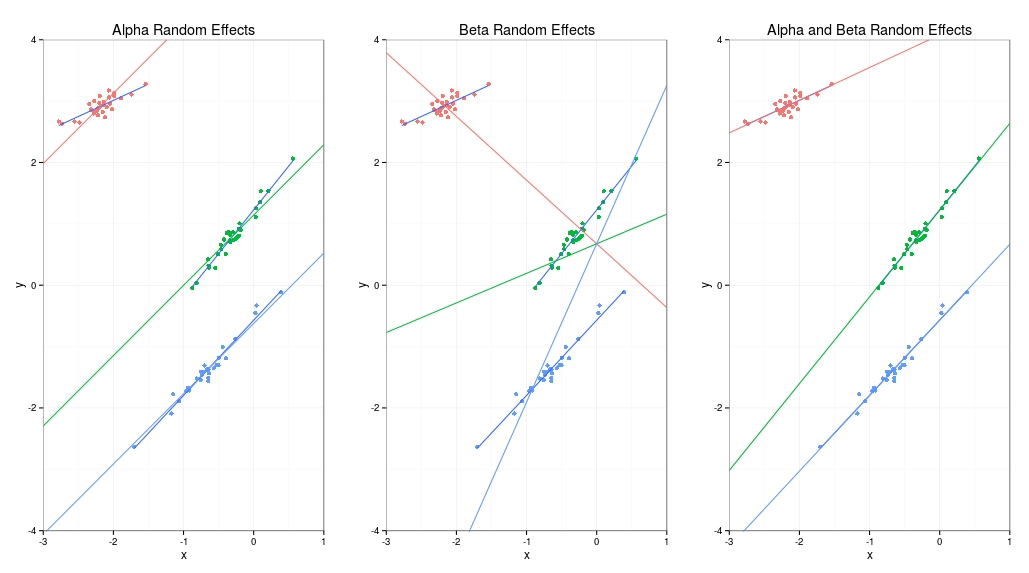
The terminology is that the top-level regression coefficients are “fixed effects” and the group-level is called “random effects”.
# > group.alpha
# [1]  4.2883814  1.2134493 -0.5410049
ranef(lmer.alpha)
# $group
# (Intercept)
# 1   3.4386106
# 2  -0.8360106
# 3  -2.6026000
ranef(lmer.beta)
# $group
# x
# 1 -1.7129750
# 2 -0.1929548
# 3  1.9059298
ranef(lmer.both)
# $group
# (Intercept)          x
# 1    2.500014 -0.5272426
# 2   -0.355365  0.3545068
# 3   -2.144649  0.1727358

fixef(lmer.alpha)
# (Intercept) x
# 1.978652    1.144952
fixef(lmer.beta)
# (Intercept) x
# 0.6749176   0.7072876
fixef(lmer.both)
# (Intercept) x
# 1.578741    1.059370
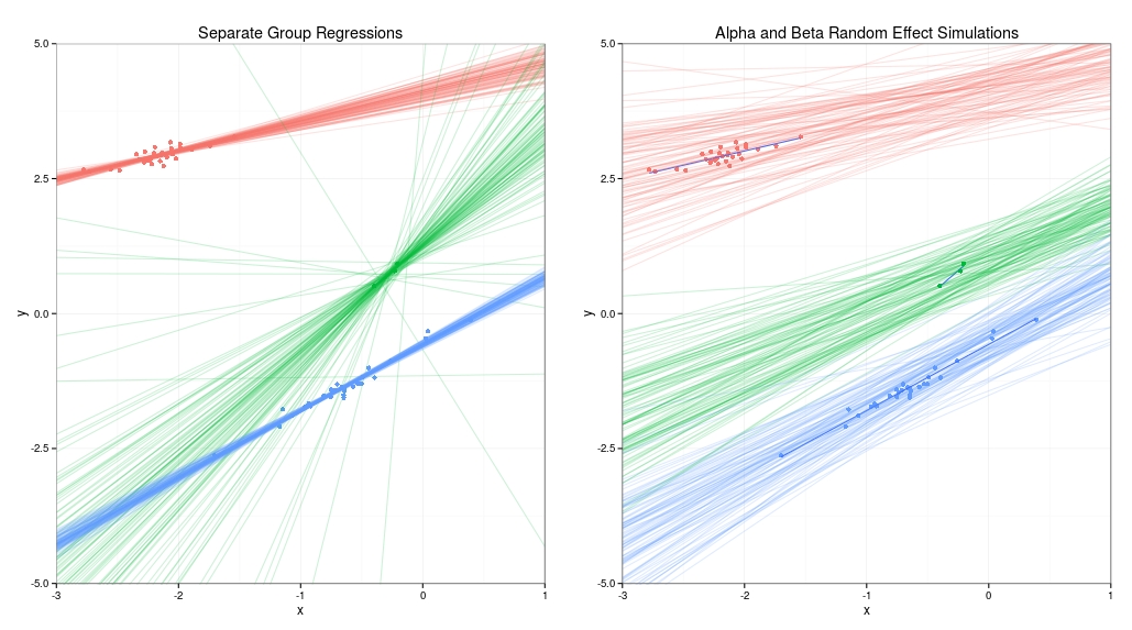
To show how the assumption that the model is hierarchical can help reduce predictive errors with a group that has a much smaller size, we can delete all but three of the data points in the second group and compare the results of no pooling and partial pooling.
# remove all but 3 data points of second group
df2 <- df[c(1:30,31:33,61:90),]
lmer.both <- lmer(y~1+x+(1+x|group),data=df2)

# plot new data in df2 with diminished group 2
g2 <- ggplot(df2) + geom_point(aes(x=x,y=y,colour=group)) +
  coord_cartesian(xlim=c(-3,1),ylim=c(-4,4)) +
  geom_smooth(aes(x=x,y=y,group=group),method=lm,se=FALSE) +
  theme_bw() + theme(legend.position="null")

# function to do rbind on matrices
rbind.mat <- function(m,n) {
  t(matrix(rbind(rep(t(m),n)),nrow=ncol(m),byrow=FALSE))
}

# simulate both alpha and beta using a hierarchical model
# sim() in the arm package simulates sigma and beta from a lm(), glm or
# in our case a merMod object produced by calling lmer()
lmer.both.sim <- sim(lmer.both)
fixef.lmer.both <- fixef(lmer.both.sim)
ranef.lmer.both <- ranef(lmer.both.sim)[[1]]
nsamples <- 100
fit.lines.both <- data.frame(matrix(ranef.lmer.both,ncol=2) +
                               rbind.mat(fixef.lmer.both,ngroups))
fit.lines.both$group <- factor(rep(1:3,each=nsamples))
colnames(fit.lines.both) <- c("intercept","slope","group")
g.sim.both <- g2 + geom_abline(aes(intercept=intercept,slope=slope,colour=group),data=fit.lines.both,alpha=.2) +
  ggtitle("Alpha and Beta Random Effect Simulations") +
  coord_cartesian(xlim=c(-3,1),ylim=c(-5,5))

# now do 3 separate linear regressions (one for each group)
# using MCMCglmm package
library(MCMCglmm)
lm.mcmc.1 <- MCMCglmm(y~1+x,data=df2[df2$group=="1",],thin = 100)
lm.mcmc.2 <- MCMCglmm(y~1+x,data=df2[df2$group=="2",],thin = 100)
lm.mcmc.3 <- MCMCglmm(y~1+x,data=df2[df2$group=="3",],thin = 100)
fit.lines.mcmc <- data.frame(rbind(lm.mcmc.1$Sol,lm.mcmc.2$Sol,lm.mcmc.3$Sol))
n <- nrow(lm.mcmc.1$Sol)
fit.lines.mcmc$group <- factor(c(rep(1,n),rep(2,n),rep(3,n)))
colnames(fit.lines.mcmc) <- c("intercept","slope","group")
g.sim.mcmc <- g2 + geom_abline(aes(intercept=intercept,slope=slope,colour=group),data=fit.lines.mcmc,alpha=.2) +
  ggtitle("Separate Group Regressions") +
  coord_cartesian(xlim=c(-3,1),ylim=c(-5,5))
g.sim.mcmc

# plot them alongside one another
multiplot(g.sim.mcmc,g.sim.both,cols=2)
The results are shown below. The graph on the left uses no pooling at all, and is just one separate linear regression per group. For the blue and red groups the lines fit the data quite well most of the time, but for the green group with just three data points the lines are all over the place because without any prior information the estimates for the slope and offset of the data are very uncertain. The graph on the right shows that for the hierarchical model the green group has drawn strength from the red and green groups. Because the model assumes that the slope and offset of all three groups is drawn from a common distribution it makes the reasonable assumption that the slope is positive. We know this is appropriate for this example because we contrived the data generating process to make it so.
For more detail I’d recommend Andrew Gelman and Jennifer Hill’s book Data Analysis using Regression and Multilevel/Hierarchical Models . There’s an amusing presentation by Gelman on Youtube called But When You Call Me Bayesian, I Know I’m Not the Only One where he talks about voting preferences in the US. And Justin Esarey has a very nice, but lengthy, video where he introduces hierarchical linear models.