The buzzword at the moment is Big Data where you have to make sense of lots of observations, but the problem we’ll discuss here is Wide Data where you have lots of observables. Another way of describing this is having too many dimensions. The question we will try to address is whether we can reduce the number of dimensions while retaining as much information as possible. That’s the goal of Principal Component Analysis (PCA).

PCA is fundamentally a rotation of the data onto a new set of axes. The rotation is chosen such that the projection of the data onto the first axis has the largest possible variance. That way when you specify the coordinate of each data point on that axis it separates the data as much as possible squeezing the maximum amount of information onto that first axis. The second axis is chosen such that it is orthogonal to the first axis but captures the maximum amount of residual variance as possible, and so on. PCA is most effective if by the time you get to the third, fourth etc. axes there is hardly any information left to describe.

The example we will use is the US yield curve. The yield curve measures interest rates at which the US Government can borrow over different periods of time (maturity) usually up to 30 years. This means we have a rate for each maturity of loan for each day in the past. Here we use 6 maturities and so we have a six-dimensional yield curve.

Mathematically we set up the problem starting with some data in a matrix M. First we standardize the data in each column by subtracting its mean and scaling such that standard deviation is equal to one, then say this matrix is X. The covariance matrix is \(\Sigma = X^T X\). What we are trying to do is diagonalize \(\Sigma\), so if \(D\) is a diagonal matrix (all the non-diagonal elements are zero) we have to find the rotation matrix \(R\) such that

The diagonal elements of \(D\) are the eigenvalues. The columns of the rotation matrix \(R\) are the eigenvectors. The function in R for performing principal component analysis is prcomp() and it returns the eigenvalues and eigenvectors as follows:

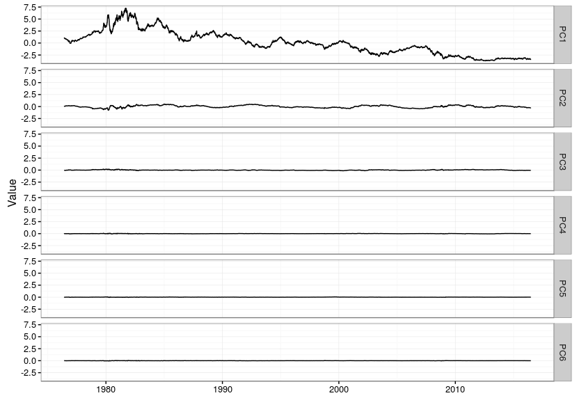
This shows how to download the yield curve history (and cache it), calculate principal components and then plot the components over time.

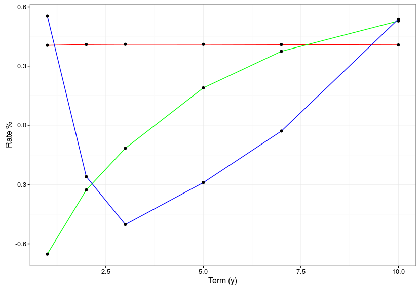
This is what the eigenvectors look like. The red flat line is the first principal component, and corresponds to a parallel move up and down in the level of the entire yield curve. The green line is the second principal component and is a steepening and flattening of the curve. The third component is a twist. In the code above you will see he comment about how much variance is captured in the first few principal components. For this data the first principal component captures a staggering 98.98%! The second component manages to capture 0.96% and the third component 0.05%, beyond that only 0.01% of variance remains.

The reason why PCA is so effective for yield curves is that rates are highly correlated. Yield curve levels in the US are at least 96% correlated and daily rate moves are at least 72% correlated. Looking at the “loadings” of the yield curves onto the eigenvectors we see that the volatility after the second principal component is almost zero because all the information about yields is squeezed into the first two principal components.

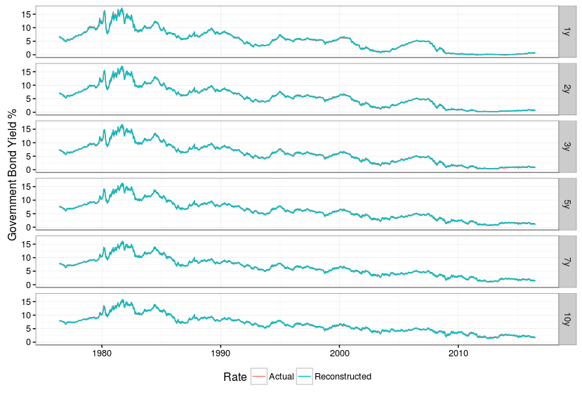
If we take the information from the first two principal components and reconstruct the entire yield curve we can assess how much information we have lost by throwing away four dimensions. The answer in this case is “not much”. The original and reconstructed rates lie almost exactly on top of one another.

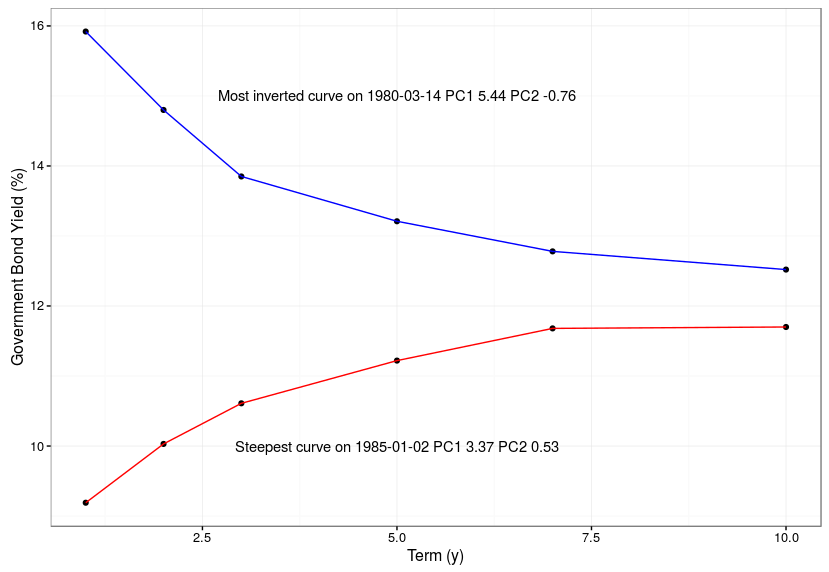
We can take a look at the curves on two days when the second principal component (steepness) was at is largest and smallest values. As you can see the curve was either inverted or strongly upward sloping on these days.