Here we explore smart beta and how to build portfolios which implement smart beta in R. Smart beta is what people call algorithms that construct portfolios that are intended to beat market cap weighted benchmarks without a human selecting stocks and bonds. So we will begin by explaining what market cap benchmarks do, what is meant by alpha and beta, then show how to easily build smart beta portfolios in R.
Using ETFs it is now possible to track whole stock markets, so if you buy the ETF called SPY you would be buying a portfolio containing the largest 500 stocks in the US. Alternatively you could try and earn a return that is higher than the market, or pay a fund manager to do so, and the margin by which they beat the market is called alpha. Another pair of words that describe these two approaches is active and passive investing: active means a team of humans is paid to beat an index like the S&P 500, and passive means you just buy and track the S&P 500.
Passively tracking a market is easy, you simply buy a portfolio of assets that match the weights of a stock market index. Consistently outperforming the market and generating alpha is extremely difficult. Few active fund managers outperform the index by more than their fees. For example see page 4 of this report by S&P that systematically tracks fund performance. They find underperfomance over the past 10 years in 98.9% of US equity funds, 97% of emerging market funds and 97.8% of global equity funds. Funds that track markets such as ETFs are beta strategies and earn small fees, usually less than 0.4% of your investment per year, whereas funds that pay humans to try to beat markets by generating alpha charge high fees, often 1% per year or higher.
The words alpha and beta come from the capital asset pricing model from which we get this simple equation relating expected asset return to a constant, \(\alpha\) plus \(\beta\) times market excess return above the risk-free rate which is usually taken to be government bond yield.
\(\mbox{expected asset return} = \alpha + \beta \times (\mbox{expected market return} – \mbox{risk free rate})\)
The aim of smart beta is to generate alpha cheaply. For example instead of buying an S&P 500 ETF you buy a low-volatility portfolio of stocks in the S&P 500. Instead of weighting the ownership of each stock by market capitalization (share price times the number of shares) this “smart beta” low volatility ETF would choose weights such that the daily combined return is diversified. There are several variants of smart beta and these might include:
- Low volatility: weights chosen such that the overall volatility of the portfolio is as low as possible.
- Momentum: trend-following strategy where weights favour assets where prices are rising assuming the trend will continue.
- Value: weights are highest for cheap assets where cheapness is measured using fundamental valuation measures.
- Risk parity: each asset contributes the same way to portfolio volatility.
The three flavours of smart beta that we touch on here are minimum variance, maximum Sharpe and risk parity. Minimum variance and maximum Sharpe are based on the idea of the efficient frontier and are the portfolios with the smallest possible risk and maximum possible risk-adjusted return. The idea behind risk parity is that portfolio weights are chosen such that each allocation contributes an equal amount of total risk to the portfolio (see here for a nice description).
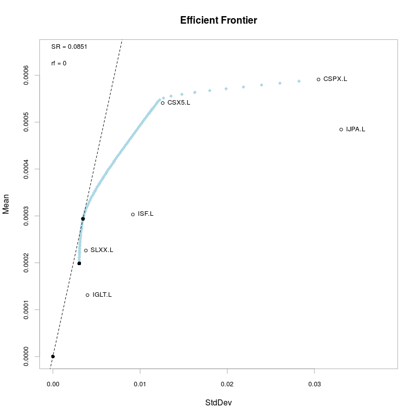
For the ETF assets we are about to consider the risk and return since 2012 are plotted on the x-axis and y-axis of this plot. Equities tend to have higher risk and higher return (lie toward the upper-right part of the plot) while fixed income carries lower volatility and lower return (bottom left hand of the plot). The blue line is the efficient frontier which, for a given return y-value (think of a horizontal line of equal return on the plot) combines the asset weights to attain the minimum risk (minimum x-value). The black dots on the efficient frontier are the minimum variance portfolio, which is the portfolio with the lowest possible volatility, and the tangency portfolio (or maximum Sharpe ratio portfolio) which has the greatest risk-adjusted excess return.
This code downloads the ETF price data.
|
1 2 3 4 5 6 7 8 9 10 11 12 13 14 15 16 17 18 19 20 21 22 23 24 25 26 27 28 29 30 31 32 33 |
library(PortfolioAnalytics) library(zoo) library(tseries) # IGLT iShares Core UK Gilts UCITS ETF # ISF iShares Core FTSE 100 UCITS ETF (Dist) # IWDA iShares Core MSCI World UCITS ETF 0.20% # CSX5 iShares Core EURO STOXX 50 UCITS ETF 0.10% # CSPX iShares Core S&P 500 UCITS ETF 0.07% # IJPA iShares Core MSCI Japan IMI UCITS ETF 0.20% # CPXJ iShares Core MSCI Pacific ex Japan UCITS ETF 0.20% # SLXX iShares Core GBP Corporate Bond UCITS ETF 0.20% # EMIM iShares Core MSCI Emerging Markets IMI UCITS ETF 0.25% ticker.list <- c("IGLT.L","ISF.L","CSX5.L","CSPX.L","IJPA.L","SLXX.L","VFEM.L") # get the time series from Yahoo z <- get.hist.quote(instrument=ticker.list[1], start="2003-01-01", end=Sys.Date(), quote="AdjClose", provider="yahoo", origin="1970-01-01", compression="d", retclass="zoo") for (ticker in ticker.list[2:length(ticker.list)]) { tmp <- get.hist.quote(instrument=ticker, start="2003-01-01", end=Sys.Date(), quote="AdjClose", provider="yahoo", origin="1970-01-01", compression="d", retclass="zoo") z <- merge.zoo(z,tmp) } colnames(z) <- ticker.list # use log returns z.logrtn <- diff(log(z)) z.logrtn <- z.logrtn[!is.na(apply(z.logrtn,1,sum)),] |
Minimum variance portfolio
For the minimum variance portfolio the marginal risk contribution for each asset is equal. If the portfolio volatility is \(\sigma\), the weight assigned to asset \(i\) and \(j\) are \(w_i\) and \(w_j\) then
\(\frac{\partial \sigma}{\partial w_i}=\frac{\partial \sigma}{\partial w_j}\)Using the PortfolioAnalytics library we build our portfolio constraints such that our portfolio is fully invested (if we have £100 to spend this is fully invested in assets) and long only (no short positions) and we use mean historic return to gauge future return and historic volatility to gauge future risk.
|
1 2 3 4 5 6 7 8 9 |
library(PortfolioAnalytics) init.portf.minvar <- portfolio.spec(assets=ticker.list) init.portf.minvar <- add.constraint(portfolio=init.portf.minvar, type="full_investment") init.portf.minvar <- add.constraint(portfolio=init.portf.minvar, type="long_only") init.portf.minvar <- add.objective(portfolio=init.portf.minvar, type="risk", name="StdDev") init.portf.minvar minvar.lo.ROI <- optimize.portfolio(R=z.logrtn, portfolio=init.portf.minvar, optimize_method="ROI",trace=TRUE) |
Maximum Sharpe ratio portfolio
One interpretation of the Sharpe ratio portfolio (alternatively called the tangency portfolio) is Sharpe parity. The weights are such that each asset’s ratio of marginal excess return \(\frac{\partial \mu}{\partial w_i} – r\) to marginal risk \(\frac{\partial \sigma}{\partial w_i}\) is equal to that of the portfolio. Here \(r\) is the risk free rate, and \(\sigma\) is the portfolio volatility.
\(\frac{\frac{\partial \mu}{\partial w_i} – r}{\frac{\partial \sigma}{\partial w_i}} = \frac{\mu – r}{\sigma}\)In matrix notation the maximum Sharpe portfolio is calculated in terms of the asset covariance matrix \(\Sigma\), asset expected return \(\mu\) and risk-free rate \(r\) as follows. This will also have negative weights, so to ensure the portfolio is long-only you have to set the negative weights to zero and re-normalize the weights (so they add up to one).
\(\frac{\Sigma ^ {-1}(\mu – r)}{1^T \Sigma ^ {-1}(\mu – r)}\)|
1 2 3 4 5 6 7 8 9 |
init.portf.maxsharpe <- portfolio.spec(assets=ticker.list) init.portf.maxsharpe <- add.constraint(portfolio=init.portf.maxsharpe, type="full_investment") init.portf.maxsharpe <- add.constraint(portfolio=init.portf.maxsharpe, type="long_only") init.portf.maxsharpe <- add.objective(portfolio=init.portf.maxsharpe, type="return", name="mean") init.portf.maxsharpe <- add.objective(portfolio=init.portf.maxsharpe, type="risk", name="StdDev") maxSR.lo.ROI <- optimize.portfolio(R=z.logrtn, portfolio=init.portf.maxsharpe, optimize_method="ROI", maxSR=TRUE, trace=TRUE) |
Risk parity portfolio
Risk parity refers to the equality (parity) of the total risk contribution of each asset. If the weight of asset i is \(w_i\) then the total risk contribution is the product of weight \(w_i\) and the marginal risk contribution \(\frac{\partial \sigma}{\partial w_i}\), where \(\sigma\) is portfolio volatility. In summary:
\(w_i \frac{\partial \sigma}{\partial w_i} = w_j \frac{\partial \sigma}{\partial w_j}\)where the marginal risk contribution is the matrix product of the covariance matrix and portfolio weights scaled by portfolio volatility
\(\frac{\partial \sigma}{\partial w_i} = \frac{\Sigma w}{\sqrt{w^T \Sigma w}}\)|
1 2 3 4 5 6 7 8 9 10 11 12 13 14 15 16 17 18 19 20 21 22 23 24 25 26 27 28 29 30 31 32 33 34 35 |
# objective function eval_f <- function(w,cov.mat,vol.target) { vol <- sqrt(as.numeric(t(w) %*% cov.mat %*% w)) marginal.contribution <- cov.mat %*% w / vol return( sum((vol/length(w) - w * marginal.contribution)^2) ) } # numerical gradient approximation for solver eval_grad_f <- function(w,cov.mat,vol.target) { out <- w for (i in 0:length(w)) { up <- dn <- w up[i] <- up[i]+.0001 dn[i] <- dn[i]-.0001 out[i] = (eval_f(up,cov.mat=cov.mat,vol.target=vol.target) - eval_f(dn,cov.mat=cov.mat,vol.target=vol.target))/.0002 } return(out) } std <- apply(z.logrtn,2,stdev) cov.mat <- cov(z.logrtn) x0 <- 1/std/sum(1/std) res <- nloptr( x0=x0, eval_f=eval_f, eval_grad_f=eval_grad_f, eval_g_eq=function(w,cov.mat,vol.target) { sum(w) - 1 }, eval_jac_g_eq=function(w,cov.mat,vol.target) { rep(1,length(std)) }, lb=rep(0,length(std)),ub=rep(1,length(std)), opts = list("algorithm"="NLOPT_LD_SLSQP","print_level" = 3,"xtol_rel"=1.0e-8,"maxeval" = 1000), cov.mat = cov.mat,vol.target=.02 ) # total contributions to risk are equal res$solution * cov.mat %*% res$solution # adding total contributions gives total risk parity portfolio volatility sum(res$solution * cov.mat %*% res$solution) res$solution %*% cov.mat %*% res$solution |
We can compare minimum variance, maximum Sharpe and risk parity weights. Notice that the minimum variance portfolio tends to assign high weights to low volatility assets i.e. fixed income, and in particular UK government bonds (IGLT.L) which make up almost 2/3 of the portfolio. UK corporate credit (SLXX.L) gets about a fifth of the portfolio. Amongst equities only the FTSE gets significant weight of 14%. The maximum Sharpe portfolio has a slightly higher risk appetite with a heavy 79% weighting in UK corporate bonds and 18% in the Eurostoxx 50 (CSX5.L).
|
1 2 3 4 5 6 7 8 9 10 11 12 |
df <- data.frame(cbind(MinVariance=minvar.lo.ROI$weights ,MaxSharpe=maxSR.lo.ROI$weights ,RiskParity=res$solution)) > round(df,2) MinVariance MaxSharpe RiskParity IGLT.L 0.62 0.00 0.38 ISF.L 0.14 0.00 0.10 CSX5.L 0.05 0.18 0.08 CSPX.L 0.01 0.02 0.04 IJPA.L 0.00 0.01 0.04 SLXX.L 0.17 0.79 0.30 VFEM.L 0.00 0.00 0.05 |