See the DLM for stocks page for an introduction to dynamic linear models. Here we can apply the same library but wrapped up in a convenient function called dlm.rolling.regression() which takes only two parameters, two or more independent variables in X and the single dependent variable in y. To test the function and demonstrate how it is used I generate a time-varying regression where I deliberately let the coefficients drift in a random walk over time. Then we can see how well the DLM performs fitting the time-varying regression using a Kalman filter.
Here’s the data generation bit. We have one dependent variable, y, and two dependent variables.
|
1 2 3 4 5 6 7 8 9 10 11 12 13 14 15 16 17 18 19 20 21 22 23 24 25 26 27 28 29 30 |
library(zoo) library(dlm) n <- 1000 set.seed(123) # beta is [n x 3] # all three coefficients are N(0,sd.beta) random walks sd.beta <- 0.4 sd.obs <- 1 beta0 <- 10 + diffinv(rnorm(n,sd=sd.beta))[1:n] beta1 <- 3 + diffinv(rnorm(n,sd=sd.beta))[1:n] beta2 <- -5 + diffinv(rnorm(n,sd=sd.beta))[1:n] beta <- cbind(beta0,beta1,beta2) # generate data, X is [n+1 x 2] # this is the design matrix so first column is the "constant" which is just 1's # column 2 and 3 are the x1 and x2 data X <- matrix(c(rep(1,n),rnorm(n*2)),nrow=n,ncol=3) colnames(X) <- c("c","x1","x2") plot(zoo(X),typ="l") # y is n x 1 # this is the dependent variable # at each point in time y_t = beta_t * x_t y <- matrix(NA,nrow=n,ncol=1) for ( i in 1:n) { y[i] <- sum(beta[i,] * X[i,]) + rnorm(1,sd=sd.obs) } data.df <- data.frame(cbind(X,y=y)) colnames(data.df)[4] <- "y" # very roughly pulls out approximate answer y ~ 10 + 3 x_1 - 5 x_2 lm(y~x1+x2,data=data.df) |
Now we can create a fairly generic function that wraps up the DLM code. This firstly estimates the observable and state variable volatility using an MLE estimate, then performs the filtration. Finally we plot the filtrations and confidence limits.
|
1 2 3 4 5 6 7 8 9 10 11 12 13 14 15 16 17 18 19 20 21 22 23 24 25 26 27 28 29 30 31 32 33 34 35 36 37 38 39 40 41 42 43 44 45 46 47 48 49 50 51 52 53 54 55 56 57 58 59 60 61 62 63 64 65 66 67 68 69 70 71 72 73 |
library(ggplot2) library(reshape2) # X contains 2 or more independent variables # y contains a single dependent variable # make sure that length(y) == nrow(X) dlm.rolling.regression <- function(X,y) { # need to build a DLM regression model in this function # so that we can tune the DLM state variance and observation variance # x[1] is the logarithm of the dependent variable's variance # x[2:4] are the logarithms of the independent variable variances (beta[,1], beta[,2] and beta[,3]) buildRegression <- function(x) { return(dlmModReg(X,addInt = FALSE,dV = exp(x[1]),dW = exp(x[2:length(x)]))) } # find MLE estimate of model variances dlm.mle <- dlmMLE(y = y, parm = c(log(sd(y)),log(rep(1,ncol(X)))), build = buildRegression) # build the model using these MLE estimates mle.model <- buildRegression(dlm.mle$par) # filtration using MLE estimates for V and W dlm.filter <- dlmFilter(y,mle.model) # confidence limits for state variables # extract std errors - dlmSvd2var gives list of MSE matrices # U.C and D.C are SVD of variances of estimation errors (we use these) # U.R and D.R are SVD of variances of prediction errors mse.list = dlmSvd2var(dlm.filter$U.C, dlm.filter$D.C) # instead of an array of covariance matrices we take just the diagonals se.mat = t(sapply(mse.list, FUN=function(x) sqrt(diag(x)))) # result data frame contains the following columns # 1 time index # 2 filtered values of constant term # 3 lower confidence interval of constant term (approx 5th percentile assuming normality) # 4 upper confidence interval of constant term (approx 95th percentile assuming normality) # 5 filtered values of beta for first independent variable # 6 lower confidence interval of first independent variable (approx 5th percentile assuming normality) # 7 upper confidence interval of first independent variable (approx 95th percentile assuming normality) # ... for cols 5 to 7 for each independent variable in X # column names and time index are taken from X g.df <- data.frame(t=time(X)) i.res <- 2 for (i.col in 1:ncol(dlm.filter$m)) { g.df[,i.res] <- dlm.filter$m[-1,i.col] colnames(g.df)[i.res] <- colnames(X)[i.col] g.df[,i.res+1] <- dlm.filter$m[-1,i.col] - 1.96 * se.mat[-1,i.col] colnames(g.df)[i.res+1] <- paste(colnames(X)[i.col],".lower",sep="") g.df[,i.res+2] <- dlm.filter$m[-1,i.col] + 1.96 * se.mat[-1,i.col] colnames(g.df)[i.res+2] <- paste(colnames(X)[i.col],".upper",sep="") i.res <- i.res + 3 } return(g.df) } # call function rr <- dlm.rolling.regression(X = X, y = y) # plot the results showing filtration with estimation error bands g <- ggplot(rr[4:nrow(rr),]) + xlab("Time") + ylab("Time-varying regression coefficients") + theme_bw() g.palette <- rainbow(n=ncol(X)) names(g.palette) <- colnames(X) for (dep.name in colnames(X)) { g <- g + geom_ribbon(aes_string(x="t" ,ymin=paste(dep.name,".lower",sep="") ,ymax=paste(dep.name,".upper",sep="")) ,alpha=.2,fill=g.palette[dep.name],alpha=0.4) + geom_line(aes_string(x="t",y=dep.name),color="red",size=.1) } g + geom_line(data=data.frame(cbind(t=1:n,beta0)),mapping=aes(x=t,y=beta0),size=1,col="red") + geom_line(data=data.frame(cbind(t=1:n,beta1)),mapping=aes(x=t,y=beta1),size=1,col="green") + geom_line(data=data.frame(cbind(t=1:n,beta2)),mapping=aes(x=t,y=beta2),size=1,col="blue") |
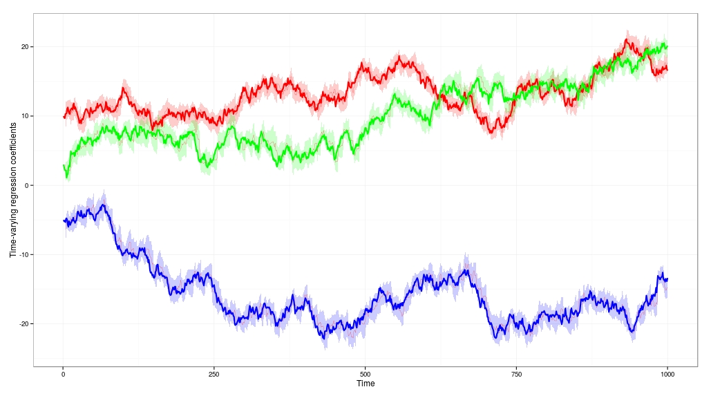
This is what the result looks like. You can see the thick red, green and blue lines are the true values of the time-varying coefficients. The Kalman filter in the DLM does a good job of dynamically tracking the coefficients as they drift. The true value of the coefficients lies within the error bands almost all of the time.